Generative AI · Deep Learning Python · PyTorch · Flask Live on HuggingFace Spaces

Train a Generative Model from Scratch — Then Explore Its Mind in Real Time

A fully interactive deep learning playground where you can configure and train a VAE on MNIST from scratch, then navigate its latent space with sliders, compare reconstructions side-by-side, and generate new digit images — all inside a single web interface backed by a PyTorch training loop.

Industry Project · 2025 Noorchenarboo 5-Tab Interactive App MNIST · 60,000 samples
2-D
Latent space — fully visualisable as a scatter manifold
60K
MNIST samples — 10K subset used for fast interactive training
5
Interactive tabs: Train, Architecture, Latent, Reconstruct, Generate
Real-time
Live loss curve & epoch progress streamed to the browser
Live
Deployed on HuggingFace Spaces — no local setup needed
How It Works

From Pixel to Latent Point and Back

A VAE learns to compress each 28×28 MNIST digit into a two-number coordinate in "latent space", then reconstruct the original from that coordinate. Because the latent space is regularised to be smooth and Gaussian, you can pick any coordinate — even one never seen during training — and the decoder will generate a plausible-looking digit. This page lets you watch every step of that process unfold in real time.

🖼️
MNIST Input
28×28 image flattened to 784-D vector
🔒
Encoder FC
784 → 400 hidden units (ReLU)
🎲
Reparameterise
μ & log σ² → z = μ + σ·ε
🔓
Decoder FC
2 → 400 → 784 (Sigmoid output)
Generated Digit
Reconstructed or freshly sampled image
💡

Why the Reparameterisation Trick Matters

Sampling from a distribution is non-differentiable — backpropagation can't flow through a random node. The trick rewrites the sample as z = μ + σ · ε where ε ∼ 𝒩(0,I), moving randomness into a fixed input ε and making μ and σ trainable by gradient descent. Without it, VAEs simply wouldn't train.

Feature Breakdown

Five Interactive Tabs, One Unified Playground

⚡ Training
Live Training Dashboard
Set epochs, batch size, learning rate, hidden dim, and latent dim. A progress bar and loss curve update every 600 ms as the model trains in a background thread — no page reloads.
BackendPython threading
Poll interval600 ms
🏗️ Architecture
Network Topology Viewer
Visual layer-by-layer diagram of the encoder, reparameterisation step, and decoder. Updates dynamically when you change hyperparameters, alongside the ELBO loss formula breakdown.
LossBCE + KL divergence
Dims784 → H → L → H → 784
🌐 Latent Space
2-D Manifold Scatter Plot
Encodes 10,000 MNIST test images and plots their μ coordinates, coloured by digit class. Tight, separated clusters indicate a well-structured latent representation.
Points10,000 encoded digits
ColourClass 0–9 (tab10)
🔁 Reconstruction
Side-by-Side Comparison
Randomly samples 10 MNIST images, encodes and decodes them, then displays originals and reconstructions in a two-row grid. Slight blurriness reveals the smoothing effect of BCE loss.
Samples10 random per click
Grid layout2 rows × 10 columns
✨ Generation
Latent Space Navigation
Two sliders (Z₁ and Z₂, range −3 to +3) let you walk through the latent manifold and instantly decode any coordinate into a digit image, or generate a 15×15 grid of the full space.
Slider range−3.0 to +3.0
Grid size15 × 15 = 225 points
⚙️ Engineering
Thread-safe Flask API
Training runs in a daemon thread; all five endpoints (/start_training, /latent_space, /reconstruction, /generate, /generate_grid) are stateless REST calls with base64-encoded PNG responses.
Endpoints7 REST routes
OutputBase64 PNG images
Architecture Detail

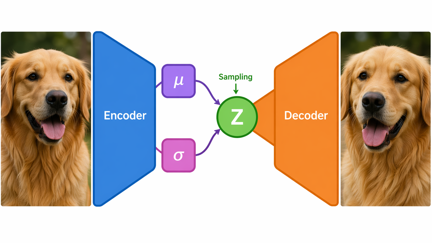
VAE Layer Diagram & Loss Decomposition

Input · 784-D
28×28 flattened pixel values (0–1 normalised)
Encoder FC · 400-D (configurable)
Linear(784, H) → ReLU
↓ split ↓
μ head & log σ² head · 2-D (configurable)
Two independent Linear(H, L) heads
↓ reparameterise ↓
Latent vector z · 2-D
z = μ + exp(½ log σ²) · ε  ·  ε ∼ 𝒩(0, I)
Decoder FC · 400-D (configurable)
Linear(L, H) → ReLU
Output · 784-D
Linear(H, 784) → Sigmoid → pixel probabilities

ELBO Loss (Evidence Lower Bound)

ℒ = ℒ_recon + KL

Reconstruction (Binary Cross-Entropy, sum)

ℒ_recon = −Σ [ x·log x̂ + (1−x)·log(1−x̂) ]

KL Divergence (closed-form Gaussian)

KL = −½ Σ [ 1 + log σ² − μ² − σ² ]

Configurable Hyperparameters

ParameterDefault
Epochs30
Batch size128
Learning rate1e-3 (Adam)
Hidden dim (H)400
Latent dim (L)2
🎯

Why 2-D as the Default Latent Dimension?

With latent dim = 2, the entire manifold becomes a 2-D scatter plot you can inspect with the naked eye. Clusters for each digit class emerge naturally from the KL regularisation. Increasing to 5, 10, or 20 dims improves reconstruction sharpness and loses interpretable 2-D structure — the app lets you explore that trade-off interactively. Higher dims improve fidelity; 2-D maximises interpretability.

Interactive Explorer

Visualise VAE Concepts Without Running the App

Select a view below to see illustrative examples of what each tab in the live app produces after training.

Each cell represents a region of the 2-D latent space. After training, digits of the same class cluster together — the VAE has learned to organise the latent manifold semantically.

Stylised representation of the 2-D latent space; colour encodes digit class (0–9).

Top row: original MNIST samples. Bottom row: VAE reconstructions decoded from the 2-D latent code. Slight blurriness is expected — BCE loss smooths pixel predictions toward the mean.

Illustrative reconstruction comparison. Live app uses actual PyTorch model outputs.

In the live app, two sliders control Z₁ and Z₂ (each from −3 to +3). The decoder maps that coordinate to a digit image in real time. Moving across the manifold smoothly interpolates between digit classes.

Five sample (Z₁, Z₂) coordinates and their decoded digit representation. The live app lets you explore any point with sliders.

Training Dynamics

Expected Training Behaviour

ELBO Loss Curve
Latent Cluster Quality
Latent Dim Trade-off

Typical ELBO loss over 30 epochs on the 10,000-sample MNIST subset with LR=1e-3 and hidden dim=400. Loss drops sharply in early epochs as the decoder learns basic digit structure, then flattens as fine detail is refined.

Approximate fraction of digit classes that form visually distinct latent clusters, measured by inter-cluster distance. Most classes separate by epoch 10; digits 4/9 and 3/5 remain closest due to visual similarity.

Trade-off between reconstruction quality (lower BCE = better) and latent interpretability as latent dimension increases from 2 to 20. The 2-D default is chosen to maximise visual interpretability at a small quality cost.

Design Decisions

Three Engineering Choices That Define This App

🔄
Non-blocking training
Training runs in a Python daemon thread so the UI stays fully interactive — you can switch tabs, inspect the architecture, and watch the live loss curve while training proceeds.
🗜️
Base64 image API
Every visualisation (loss curve, latent scatter, reconstruction grid) is rendered server-side by Matplotlib, encoded as base64 PNG, and injected into the DOM — zero external image hosting needed.
🎛️
Fully configurable dims
Latent dim and hidden dim are runtime hyperparameters. Changing them re-instantiates the VAE and updates the architecture diagram labels live — the UI always reflects the model you're actually training.